Understanding quantum bit notation

(Cover photo by Mark Garlick on Science Photo Library.)

Quantum computers are going to accelerate drug discovery, change the way we encrypt our information, and much more. If you haven’t heard of quantum computing yet, here’s a video that provides a nice introduction.

This article breaks down how we mathematically express qubits (quantum bits) and explains why each notation works.

Refresher on superposition: in classical computing, bits can only take on boolean values (0 or 1 and nothing in-between). But a qubit can be in a superposition of $\vert0\rangle$ and $\vert1\rangle$. (For now, let the symbols “$\vert$” and “$\rangle$” just be indicators that a value is related to a quantum object.) Qubits in superposition have some chance of “collapsing” to $\vert0\rangle$ and some chance of collapsing to $\vert1\rangle$ when measured.

• Whenever a qubit is measured, it must collapse to $\vert0\rangle$ or $\vert1\rangle$
• After a qubit collapses to $\vert0\rangle$ or $\vert1\rangle$, it does not go back into superposition. If it collapsed to $\vert0\rangle$, it is now $\vert0\rangle$.

Expressing 1 qubit

Expanded notation for 1 qubit

Let’s say we have a qubit, $\vert\psi\rangle$. Perhaps you have seen expanded notation:

$$\ket{\psi}=a\ket0+b\ket1$$

This representation uniquely describes the qubit’s superposition:

• $a^2$ is the probability that $\vert\psi\rangle$ will collapse to $\vert0\rangle$ when measured
• $b^2$ is the probability that $\vert\psi\rangle$ will collapse to $\vert1\rangle$ when measured

(Technically, $a^2$ and $b^2$ are relative probabilities. They’re scaled so that $a^2 + b^2 = 100\%$. They’re squared because they could be negative.)

For example, this qubit has a 50% chance of collapsing to $\vert0\rangle$ or $\vert1\rangle$ when measured:

$$\ket{\psi_1}=\sqrt{0.5}\cdot\ket{0}+\sqrt{0.5}\cdot\ket{1}$$

And this qubit has a 100% chance of collapsing to $\ket1$ when measured:

$$\begin{align*}\ket{\psi_2}&=0\cdot\ket{0}+1\cdot\ket{1}\\&=\ket{1} \end{align*}$$

This helps to answer the question, what do the $\vert1\rangle$ and $\vert0\rangle$ represent?

• Example #2 (above) shows that $\vert1\rangle$ represents a qubit will certainly collapse to $\vert1\rangle$ (because it already is $\vert1\rangle$).
• By similar logic, $\vert0\rangle$ represents a qubit that always collapses to (or “has collapsed to”) $\vert0\rangle$.

This builds intuition about expanded notation. Some qubit, $a\ket0+b\ket1,$ is a combination of the fundamental $\vert0\rangle$ and $\vert1\rangle$ states, with some chance of becoming $\vert0\rangle$ or $\vert1\rangle$ (collapsing upon measurement).

Vector notation for 1 qubit

There exists another way to express qubits, which involves vectors. If you’ve never seen vectors or matrices, you should check out this introduction.

To start, let’s define $\vert0\rangle$ and $\vert1\rangle$ in terms of vectors:

$$\begin{align*}\ket{0}&=\begin{pmatrix}1 \\ 0\end{pmatrix}\\\ket{1}&=\begin{pmatrix}0 \\ 1\end{pmatrix}\end{align*}$$

We will get back to why these definitions make sense. For now, let’s see how they let us rewrite a qubit:

$$\begin{align*}\ket{\psi}&=a\ket{0}+b\ket{1}\\ &=a\begin{pmatrix}1\\0\end{pmatrix}+b\begin{pmatrix}0\\1\end{pmatrix}\\ &=\begin{pmatrix}a\\0\end{pmatrix}+\begin{pmatrix}0\\b\end{pmatrix}\\ &=\begin{pmatrix}a\\b\end{pmatrix} \end{align*}$$

So the qubit $\vert\psi\rangle$ can be expressed as just one vector of two numbers:

$$\psi=\begin{pmatrix}a\\b\end{pmatrix}$$

And note that $a$ and $b$ still represent the coefficients of $\vert0\rangle$ and $\vert1\rangle$ (all we did was mathematically simplify the expression).

• $a^2$ is still the probability that the qubit will collapse to $\vert0\rangle$ when measured
• $b^2$ is still the probability that the qubit will collapse to $\vert1\rangle$ when measured

For example, this qubit has a 50% chance of collapsing to $\vert0\rangle$ or $\vert1\rangle$ when measured:

$$\ket{\psi_3}=\begin{pmatrix}\sqrt{0.5}\\\sqrt{0.5}\end{pmatrix}$$

This qubit has a 100% chance of collapsing to $\vert1\rangle$ when measured:

$$\ket{\psi_4}=\begin{pmatrix}0\\1\end{pmatrix}$$

But a qubit that has a 100% chance of collapsing to $\vert1\rangle$ is just the qubit $\vert1\rangle$. So Example #4 (above) shows us the following:

$$\ket{\psi_4}=\begin{pmatrix}0\\1\end{pmatrix}=\ket1$$

Similarly, the vector below represents a qubit with a 100% chance of collapsing to $\vert0\rangle$ when measured, so it is $\vert0\rangle$:

$$\ket{\psi_5}=\begin{pmatrix}1\\0\end{pmatrix}=\ket0$$

And these are the two definitions that we began with:

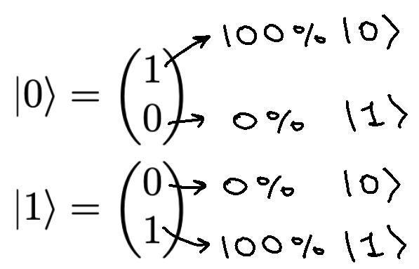
Note, it just happens that $1^2 = 100\%$ and $0^2 = 0\%$, so it seems the values weren’t squared.

Now you see how the initial definitions of $\vert0\rangle$ and $\vert1\rangle$ make sense — they uphold the following rule:

• $(\text{top num})^2$ = probability the qubit collapses to $\vert0\rangle$ when measured
• $(\text{bottom num})^2$ = probability the qubit collapses to $\vert1\rangle$ when measured

But what if $\vert\psi\rangle$ were comprised of more than one qubit?

Expressing 2+ qubits

Expanded notation for 2+ qubits

We can use expanded notation in a very similar manner. Note, though, that each additional qubit doubles the number of fundamental states:

1 qubit, $2^1=2$ states:

$$\ket0,\ket1$$

2 qubits, $2^2=4$ states:

$$\ket{00}, \ket{01}, \ket{10}, \ket{11}$$

3 qubits, $2^3=8$ states:

$$\ket{000}, \ket{001}, \ket{010}, \ket{011}, \ket{100}, \ket{101}, \ket{110}, \ket{111}$$

(In general, an $n$-qubit system can be in a superposition of $2^n$ states.)

So, for example, a 4-qubit system could be written in expanded notation as follows (note, $2^4$ states need to be represented):

$$\begin{align*}\ket{\psi}&=a\ket{0000}+b\ket{0001}+c\ket{0010}+d\ket{0011}\\ &+e\ket{0100}+f\ket{0101}+g\ket{0110}+h\ket{0111}\\ &+j\ket{1000}+k\ket{1001}+l\ket{1010}+m\ket{1011}\\ &+n\ket{1100}+o\ket{1101}+p\ket{1110}+q\ket{1111}\\\end{align*}$$

As you can see, expanded notation becomes tedious to write. But there exists a more compact way to represent qubits!

Vector notation for 2+ qubits

A multi-qubit system can also be represented as a vector. For simplicity, let’s consider a 2-qubit system (we write $\vert00\rangle$ to $\vert11\rangle$ in ascending binary order):

$$\begin{align*}\ket{\psi}&=a\ket{00}+b\ket{01}+c\ket{10}+d\ket{11}\\\end{align*}$$

Let’s name the two qubits in our 2-qubit system, qubit 1 and qubit 2. Coloring the equation will help visualize this (qubit 1 is in red, qubit 2 is in blue):

$$\begin{align*}\ket{\psi}&=a\ket{\textcolor{red}{0}\textcolor{blue}{0}}+b\ket{\textcolor{red}{0}\textcolor{blue}{1}}+c\ket{\textcolor{red}{1}\textcolor{blue}{1}}+d\ket{\textcolor{red}{1}\textcolor{blue}{1}}\\\end{align*}$$

For example, the state $\vert01\rangle$ is equivalent to

• qubit 1 (red) in state $\vert0\rangle$
• qubit 2 (blue) in state $\vert1\rangle$

We already know how to write the two qubits of $\vert\psi_6\rangle$ in vector notation:

$$\begin{align*}\text{qubit 1 of $\ket{\psi}$} &= \begin{pmatrix}x\\y\end{pmatrix} \\ \text{qubit 2 of $\ket{\psi}$} &= \begin{pmatrix}z\\w\end{pmatrix}\end{align*}$$

• $x^2 =$ probability that qubit 1 collapses to $\vert0\rangle$ when measured
• $y^2 =$ probability that qubit 1 collapses to $\vert1\rangle$ when measured
• $z^2 =$ probability that qubit 2 collapses to $\vert0\rangle$ when measured
• $w^2 =$ probability that qubit 2 collapses to $\vert1\rangle$ when measured

While the coefficients here are not $a$, $b$, $c$, and $d$, they’re related to $a$, $b$, $c$, and $d$, as we will now show. Note that the probability that \vert\psi₆\rangle collapses to $\vert00\rangle$ when measured can be represented in two ways:

1. It is $a^2$ by definition. (Remember, $\ket\psi = a\vert00\rangle + \cdots$)
2. It is also $x^2\cdot z^2$ since collapsing to $\vert00\rangle$ means:
   • qubit 1 collapses to$\vert0\rangle$ (with probability $x^2$) and
   • qubit 2 collapses to $\vert0\rangle$ (with probability $z^2$)

So it turns out that:

$$\begin{align*}a^2&=x^2\cdot z^2\\ a&=xz\end{align*}$$

Similarly, the probability that $\vert\psi_6\rangle$ collapses to $\vert01\rangle$ when measured can be represented in two ways:

• $b^2$ (remember, $\vert\psi_6\rangle = \cdots + b\vert01\rangle + \cdots$ )
• $x^2\cdot w^2$ (qubit 1 collapses to $\vert0\rangle$ and qubit 2 collapses to $\vert1\rangle$)

This yields

$$\begin{align*}b^2&=x^2\cdot w^2\\ b&=xw\end{align*}$$

And the same can be done for $\vert\psi_6\rangle$ collapsing to $\vert10\rangle$ to show

$$\begin{align*} c^2&=y^2\cdot z^2\\ c&=yz \end{align*}$$

or $\vert\psi_6\rangle$ collapsing to $\vert11\rangle$ to show

$$\begin{align*} d^2&=y^2\cdot w^2\\ d&=yw \end{align*}$$

So we have

$$\begin{align*}a&=xz\\ b&=xw\\ c&=yz\\ d&=yw\end{align*}$$

This relationship between $a$, $b$, $c$, $d$ and $x$, $y$, $z$, $w$ in Fig 24 will soon help us to understand the intuition behind the vector representation of $\vert\psi_6\rangle$.

To represent a system of 2+ qubits in vector notation, we take the tensor product ‘$\otimes$’ of all of the qubits (we’ll understand why further down). For now, let’s just see what happens:

$$\begin{align}\ket{\psi_6} &= \text{qubit 1}\otimes\text{qubit 2}\\ &= \begin{pmatrix}x\\y\end{pmatrix}\otimes\begin{pmatrix}z\\w\end{pmatrix}\\ &= \begin{pmatrix}xz\\xw\\yz\\yw\end{pmatrix}\\ &= \begin{pmatrix}a\\b\\c\\d\end{pmatrix} \end{align}$$

Here are the steps from above broken down:

• (2) replace qubit 1 and qubit 2 with their vector notations
• (3) compute the tensor product
• (4) rewrite in terms of $a$, $b$, $c$, $d$

Look at that! We’ve simplified a 2-qubit system to just one vector:

$$\begin{align*}\ket{\psi_6} = a\ket{00}+b\ket{01}+c\ket{10}+d\ket{11} = \begin{pmatrix}a\\b\\c\\d\end{pmatrix} \end{align*}$$

There’s something special about this vector! Notice that if you square the values of the vector from top-to-bottom, you get, $a^2$, $b^2$, $c^2$, and $d^2$. Those are the probabilities that $\vert\psi_6\rangle$ will collapse to $\vert00\rangle$, $\vert01\rangle$, $\vert10\rangle$, or $\vert11\rangle$ when measured.

That’s why we take the tensor product of the qubits—it makes the result contain all the coefficients defining the superposition. And because of the way a tensor product is calculated, the coefficients will be in the same order as they were in expanded notation!

For example, we could find the probability that $\vert\psi_6\rangle$ will collapse to $\vert01\rangle$ when measured by squaring the second item in its vector representation, shown in green:

$$\begin{align*}\ket{\psi_6} = a\ket{00}+\textcolor{ForestGreen}{b}\ket{01}+c\ket{10}+d\ket{11} = \begin{pmatrix}a\\\textcolor{ForestGreen}{b}\\c\\d\end{pmatrix} \end{align*}$$

Notice that there is no $\vert01\rangle$ in the vector representation because it is implied.

Say we are told that a 2-qubit system, $\vert\psi_7\rangle$, has a 50% chance of collapsing to $\vert00\rangle$ or $\vert11\rangle$ when measured. We can write it in vector notation as follows:

$$\begin{align*}\ket{\psi_7} = \textcolor{MidnightBlue}{\sqrt{0.5}}\cdot\ket{00}+\textcolor{ForestGreen}{0}\cdot\ket{01}+\textcolor{#FE6F5E}{0}\cdot\ket{10}+\textcolor{Plum}{\sqrt{0.5}}\cdot\ket{11} = \begin{pmatrix}\textcolor{MidnightBlue}{\sqrt{0.5}}\\\textcolor{ForestGreen}{0}\\\textcolor{#FE6F5E}{0}\\\textcolor{Plum}{\sqrt{0.5}}\end{pmatrix} \end{align*}$$

Again, the values in the vector correspond to the fundamental states in descending order (e.g., $\vert00\rangle$, $\vert01\rangle$, $\vert10\rangle$, $\vert11\rangle$ for 2 qubits). The expanded notation is no longer needed! Also, remember, the values are squared to find the coefficients.

Finally, here is what the generic 4-qubit system from Fig 16 would look like in vector notation:

$$\begin{align*}\ket{\psi}&=a\ket{0000}+b\ket{0001}+c\ket{0010}+d\ket{0011}\\ &+e\ket{0100}+f\ket{0101}+g\ket{0110}+h\ket{0111}\\ &+j\ket{1000}+k\ket{1001}+l\ket{1010}+m\ket{1011}\\ &+n\ket{1100}+o\ket{1101}+p\ket{1110}+q\ket{1111}\\ &=\begin{pmatrix}a\\b\\c\\d\\e\\f\\g\\h\\j\\k\\l\\m\\n\\o\\p\\q\end{pmatrix}\\ \end{align*}$$

While that’s a very tall vector, at least you don’t need to write out all the states from $\vert0000\rangle$ to $\vert1111\rangle$.

That’s it! Hopefully, you now have a better grasp of the notation.

What next?

Understanding qubits in vector notation becomes very helpful when you begin to work with quantum logic gates. The gates can be represented as matrices so that their interactions with qubits become matrix multiplications. If you’re interested in how that works, check out this lecture about the mathematical representation of quantum computing.